Mastering Cell References: Edit the Formula in Cell D2 so the References

Understanding Cell References in Excel

When working with formulas in Excel, it’s crucial to understand cell references. This concept allows us to manipulate and analyze data effectively in spreadsheets, ensuring accurate results. In this section, we will delve into what cell references are and the different types that exist.

In Excel, a cell reference is a way to identify and locate a specific cell or range of cells within a worksheet. It acts as a pointer that tells the formula where to look for the data it needs to perform calculations or return results. By using cell references in formulas, we can create dynamic and flexible spreadsheets that automatically update when the underlying data changes.

Cell references in Excel are made up of two components: the column letter and the row number. For example, the reference for cell A1 consists of the column letter “A” and the row number “1”. By combining these two components, we can reference any cell in the worksheet.

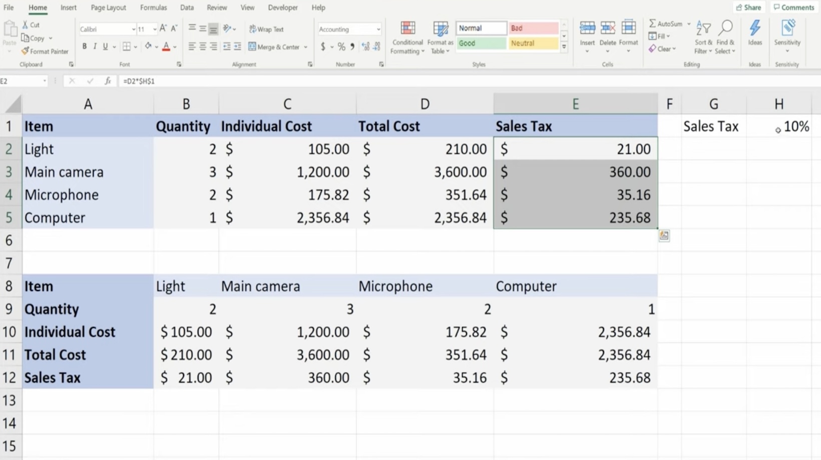
There are three types of cell references in Excel: relative references, absolute references, and mixed references. Let’s explore each type in more detail:

Relative References

Relative references are the most commonly used type of cell reference in Excel. When a formula containing a relative reference is copied to other cells, the reference adjusts based on its new location. For example, if we have a formula in cell B2 that references cell A1, when we copy the formula to cell B3, it will automatically adjust to reference cell A2.

Absolute References

Absolute references, denoted by the use of the dollar sign symbol ($), do not change when a formula is copied to other cells. This means that the reference remains fixed, regardless of its new location. To create an absolute reference, we can either add the dollar sign before the column letter (e.g., $A1) to fix the column, or before the row number (e.g., A$1) to fix the row.

Mixed References

Mixed references combine elements of both relative and absolute references. They allow us to fix either the column or the row while allowing the other component to adjust when the formula is copied. To create a mixed reference, we use the dollar sign before either the column letter or the row number, but not both.

Edit the Formula in Cell D2 so the References

Importance of Formula in Cell D2

The formula in cell D2 is a crucial element in Excel spreadsheets as it allows us to perform calculations and manipulate data efficiently. By understanding and utilizing the formula in cell D2, we can streamline our workflows and achieve accurate results. Here’s why the formula in cell D2 is important:

1. Data Analysis: The formula in cell D2 enables us to analyze data effectively. We can use mathematical operators, functions, and references to perform calculations on the data in other cells. This helps us gain insights and make informed decisions based on the analysis.
2. Automation: With the formula in cell D2, we can automate repetitive tasks. By referencing cells and applying formulas, we can create dynamic spreadsheets that automatically update when the underlying data changes. This saves us time and effort, especially when dealing with large datasets.
3. Flexibility: The formula in cell D2 allows us to create flexible spreadsheets. We can easily modify the formula to adapt to changes in data or requirements. By using relative references, absolute references, or mixed references, we can adjust the formula to suit our needs without the need for manual re-calculation.

How to Create a Formula in Cell D2

Creating a formula in cell D2 is a simple process that can be done in just a few steps. Here’s how you can do it:

1. Select Cell D2: Begin by selecting cell D2, where you want to enter the formula.
2. Start the Formula: Type an equals sign (=) in the selected cell. This indicates to Excel that you are entering a formula.
3. Enter the Formula: Enter the desired formula using mathematical operators (+, -, *, /) and functions (such as SUM, AVERAGE, MAX, MIN) to perform calculations. You can also include cell references to incorporate data from other cells.
4. Complete the Formula: Once you have entered the formula, press Enter on your keyboard to complete it. Excel will calculate the result based on the formula and display it in cell D2.
5. Copy the Formula: If you want to apply the same formula to multiple cells, you can copy the formula in cell D2 and paste it into other cells. Excel will automatically update the cell references in the formula to match the new location.

Remember, the formula in cell D2 can be as simple or as complex as you need it to be. Experiment with different formulas and functions to achieve the desired results.